Minimalist DCA in Python
2020-05-20
It’s important, as a rule of thumb, when operating or investing in a firm which produces a physical commodity, to have the ability to reliably quantify the expected future production of the commodity given the firm’s assets. In the oil and gas industry, we have many different ways to forecast future production from an oil or gas well. Some rely on detailed measurements and explicitly incorporate detailed mathematical models of flow physics. Others use whatever historical data we can scrape together and a bit of curve-fitting.
Today, we’re talking about the second kind.
Arps DCA in a Nutshell
Sophisticated approaches are great for the operator, who should have access to daily or higher-resolution rate and pressure data and a detailed understanding of the well and completion design. For us on the outside, trying to put a value on an operator’s assets, we’re usually limited to “public data”: for instance, the monthly volume data for Eddy County, New Mexico which we retrieved previously.
This nudges us toward applying empirical decline-curve analysis (DCA). DCA is all about curve-fitting: we know, from experience, the rough functional forms which should characterize the rate vs. time relation for oil and gas wells; we’ll apply optimization algorithms to find parameters to these functions which best fit the observed data. We can then use the best-fit parameters to forecast future production.
There is infinite nuance to be explored in this topic, very little of which we’ll discuss in today’s article. The short version is this: in the early 1940s, while physicists in New Mexico toiled perfecting the most destructive weapon in human history, J. J. Arps at the British-American Oil Company (now Gulf Canada) was researching and documenting a “weapon” which would arguably—eventually—result in a similarly spectacular destruction of capital in the late 2010s. Sarcasm aside, Arps published several papers which changed the oil and gas industry permanently. He documented that production from flowing oil and gas wells tended to follow one of a few different functional forms (exponential, harmonic, or hyperbolic) depending on the details of the fluid being produced and the reservoir physics. These equations were straightforward to fit to observed data even using the technology of the day (that is, graph paper).
Like atomic energy, the Arps equations can be used for both beneficial and destructive purposes. When applied with good sense by trained engineers in appropriate situations, Arps decline fits are completely adequate for forecasting production; indeed they are the most commonly used tool for estimating reserves for publicly-traded oil and gas companies. Notice the caveats. The advent of “unconventionals” (shale gas, shale oil, coalbed methane, etc.) throws a kink into the key assumptions. Specifically, without going into too much detail (ask an active reservoir engineer!), wells in these assets generally experience multiple flow regimes, each observable on an economically material timescale, which alter the functional form required to correctly fit the rate vs. time data.
That is, a hydraulically-fractured horizontal shale oil well may begin production on an apparent Arps hyperbolic decline with a b exponent of 2.0; but it may begin to follow something closer to a hyperbolic decline with a b of 0.5, or even an exponential decline, within the first year. A naïve curve fit, especially to early data, can result in a shockingly overstated estimated ultimate recovery (EUR). In my opinion, this underappreciated—especially by investors—phenomenon is responsible for a large portion of the gap between producers’ investor relations statements and reality, and the frequent reserves write-downs, in recent years.
Plenty of smart people have worked on this problem, and good solutions exist. There are a number of decline curve models which account for multiple flow regimes; for example, my friend David Fulford has published extensively on the transient hyperbolic relation as well as Bayesian techniques for fitting it probabilistically (disclosure: I’m a co-author on that one).
Unfortunately, to keep things simple today, we’ll just be using the original Arps relations. As you examine the results, look for fits which illustrate these problems. This is still a common practice in industry: you may draw your own implications.
I Will Face Guido and Walk Backwards Into Hell
…in many cultures, the python is seen as a strong and powerful creature.
–Wikipedia
Now that I’ve complained about Arps decline-curve analysis but decided to use it anyway, I’m going to do the same about Python! Engineering is, for the most part, a quantitative discipline which demands a certain degree of rigor. Naturally, we seem to have converged on learning a programming language which is pig-slow for numeric code “out of the box” and where more-or-less anything goes, with minimal facilities for automating the task of validating the correctness of our code.
As a famous Vorlon once said, “the avalanche has already begun; it is too late for the pebbles to vote”. So, given that Python seems to be the new incumbent language of engineering automation (at least it is an improvement on Excel VBA in some ways—but not all!), we’ll step through the construction of a simple Arps decline-curve forecasting system in Python. We’re going to build something at the scale that a working reservoir engineer or analyst might be able to construct as a prototype: this won’t be an “industrial grade” system, but a sketch of something that’ll get the job done to do quick evaluations of up to a few thousand wells.
This won’t, however, be the “beginner Python” you’ll frequently see in similar examples online. We are going to take more seriously the concerns of performance and correctness. To get there, we’re going to have to address some key deficiencies of the language.
Deficiency 0: Dependency Management
The Python ecosystem’s take on package management and dependency resolution is a hot mess. Most beginners learn how to pip install into the global Python’s packages directory, but that’s a recipe for pain as programs accumulate with mutually incompatible dependency versions. We’ve got a huge variety of half-baked “solutions”: venv, conda, pipenv, poetry… each with their own pain points.
We’re going to take minimalism as a virtue, and use venv to manage a virtual environment for our project. On Windows, we’ll have to take some extra steps to acquire dependencies, but it’s worth it to avoid the complexity of things like conda.
venv is the successor to the old virtualenv. It’s a relatively simple approach: copy the global Python interpreter to a new directory, set up pip and pals to install packages into that new directory, and configure the user’s environment variables to point to the new system when they run python. There are cleaner ways to do this, but at least it’s not an invasive alien ecosystem trying to take over every aspect of Python operation.
We won’t go into horrifying detail here, but I’ll provide commands to follow along on recent versions of Windows (I know reservoir engineers). You’ll want to download the latest version of Python 3—at time of writing, Python 3.8.3—for your operating system from python.org, if you don’t already have a version installed. Windows users should note that the default link goes to the 32-bit rather than 64-bit version of Python. No, I don’t know why the hell they do that. You can get the 64-bit version which you almost certainly would rather have by going here and choosing one of the “x86-64” options.
With Python properly installed, we can create a venv for our project. I like to create these in the project’s working directory with the name .venv:
python -m venv .venvNow, we can “activate” the environment with (Windows):
.venv\Scripts\activateor (Unix-likes):
source .venv/bin/activateFrom this point on (in our current shell session), everything we do will touch only the venv: python will refer to the venv’s Python interpreter; pip install will install into the venv, and so on.
Should we choose to leave the virtual environment, we can simply run:
deactivateto return to our original configuration.
Deficiency 1: Static Analysis
The next problem we’ll address is the lack of tools for ensuring the correctness of our programs. There are many approaches to program correctness, all imperfect. Historically Python’s community has encouraged a reliance on automated testing, but to quote Edsger Dijkstra:
Program testing can be used to show the presence of bugs, but never to show their absence!
Type systems are a common discipline for statically (that is, before the program is run) checking the correctness of programs with respect to desired properties. These properties might include anything from “the program never exhibits undefined behavior (i.e. crashes)” to “the program takes a finite list of input strings, parses them to integers if possible, and produces a same-length list of integers in sorted order as output”.
Fortunately, there has been significant work on “gradual typing” in recent years, resulting in the introduction of bolt-on typecheckers for “dynamic” languages like Python. The most popular is mypy, which originated at Dropbox and counts Python creator Guido van Rossum among its developers.
mypy is conservative: it implements a relatively simple type system, and allows use of an Any type to hand-wave Python idioms which can’t easily be statically typed. Nonetheless, it’s a powerful tool for catching common programming errors (including things like misspelled variable names, which aren’t usually though of as “type errors”).
We can install mypy into our virtual environment with:
pip install mypyTo typecheck a given program prog.py:
mypy prog.pyDeficiency 2: Numeric Performance
Engineering code is often “numeric”: we want to work efficiently with (approximations of) things like real numbers, vectors, matrices and so on. Python’s built-in data structures are an awkward fit for this sort of code. As an approximation to a vector or matrix, a Python list is a poor substitute for a C or Fortran style array. Python’s lists hold their elements “boxed” behind pointers, so each element access into a list of float follows at least two levels of indirection, compared to a simple calculation of (base address + index * element size) required to index into a contiguous array.
Additionally, Python’s built in numeric operations are implemented on a “scalar” basis (one value at a time) and have significant overhead due to the requirement for runtime type checking and interpretation. We can loop over sequences and apply these operations element-wise, but we’ll pay this overhead again and again for each element. We’d prefer a representation where we store a type tag along with a contiguous, homogeneous array of elements, and provide efficient compiled-code “vectorized” operations over entire arrays.
Fortunately, this exact representation is provided by numpy, the library which forms the basis for effectively all serious numerical computing in Python. numpy combines fast compiled libraries for linear algebra and array manipulation with a “Pythonic” API which lets us interact easily with optimized arrays using the same interface as Python’s built-in sequence types.
numpy is easy to install from the Python Package Index on non-Windows operating systems (with pip install numpy). Windows users will want to visit Christoph Gohlke’s site (https://www.lfd.uci.edu/~gohlke/pythonlibs/) and download the correct “wheel” for the latest version of “numpy+mkl”, depending on their Python version.
For example, at time of writing, the latest version available for 64-bit Python 3.8 is numpy-1.18.4+mkl+cp38-cp38-win_amd64.whl. Download this file, then install directly from the downloaded wheel with
pip install numpy-1.18.4+mkl+cp38-cp38-win_amd64.whlsubstituting the full path to the downloaded wheel.
We’ll also want to make use of the scipy package, which provides a variety of scientific computing tools built on numpy. Specifically, we’re going to use the library of efficient optimization routines it provides. Users on all platforms should be able to install this with:
pip install scipyWe will use matplotlib to visualize our fits.
pip install matplotlibFinally, we’d like mypy to be aware of the types provided by numpy. The numpy project doesn’t officially provide support for this yet, but the numpy-stubs repository contains their work-in-progress implementation, which we’ll install and use. We can install the package directly from GitHub with pip:
pip install git+https://github.com/numpy/numpy-stubs.gitDeficiency 3: Simple Record Types
Python supports user-defined data types through classes. Unfortunately, these often give us “too much”. Object-oriented classes combine data encapsulation and abstraction (which we want) with features like mutability, dynamic dispatch, and inheritance (which we don’t need).
This program will deal with simple data: well API numbers, rate and time arrays, and decline parameters. None of these require the more complex features of classes: in fact, we’d prefer to treat them as immutable “bags of data”; immutability is a helpful tool for correctness as it reduces the number of possible program states and prevents important program invariants from being yanked out from under us by mutation.
Python provides a few solutions to this, ranging from hand-written “record classes” to namedtuple. We’ll use the relatively new dataclasses package, which is included with Python since version 3.7.
dataclasses provides a decorator which we can use to turn a class containing member definitions with type annotations into a fully featured “record class” similar to what we might write by hand. It will automatically write constructors (__init__), display functions (__repr__), structural equality comparisons (__eq__), and other common functions for us from our annotated member definitions. We can also use the frozen feature to achieve (alas, dynamically-enforced) immutability.
With our tools (venv, mypy, numpy, scipy, matplotlib, dataclasses) in place, we are now ready to begin implementation. In this article, we’ll present the implementation a piece at a time, not necessarily in the order in which they occur in the final product but rather in roughly the order we might write them. The completed program can be previewed on GitHub at https://github.com/derrickturk/pydca.
Implementation I: Forecasting
Let’s begin by writing a dataclass which describes a single Arps hyperbolic fit. The hyperbolic decline subsumes the harmonic (b = 1) and exponential (b = 0) declines as special cases.
We’ll need to store the three decline parameters (qi, Di, and b), and provide functions for evaluating the rate vs. time relation.
import numpy as np
import dataclasses as dc

@dc.dataclass(frozen=True)
class ArpsDecline:
    qi: float # daily rate
    Di_nom: float # nominal annual decline
    b: float # unitless exponent

    def __post_init__(self):
        if self.qi < 0.0:
            raise ValueError('Negative qi')
        if self.Di_nom < 0.0:
            raise ValueError('Negative Di_nom')
        if self.b < 0.0 or self.b > 2.0:
            raise ValueError(f'Invalid b: {self.b}')

    # time (years)
    # returns (daily rate)
    def rate(self, time: np.ndarray) -> np.ndarray:
        if self.b == 0:
            return self.qi * np.exp(-self.Di_nom * time)
        elif self.b == 1.0:
            return self.qi / (1.0 + self.Di_nom * time)
        else:
            return (
              self.qi / (1.0 + self.b * self.Di_nom * time) ** (1.0 / self.b)
            )
The math itself isn’t very interesting. It’s a direct translation of the Arps equations for the hyperbolic, harmonic, and exponential cases, dispatched on the value of b. We use ordinary Python arithmetic operators (*, **, etc.), but rely on the fact that numpy overloads these for arrays to provide efficient vectorized operations.
I’ve chosen to store a nominal decline rather than an effective decline, because that’s what the Arps equations actually work with. For a good reference on how to convert between nominal and the various flavors of effective decline, see SPEE REP #6. Throughout the code, we’ll use the convention that rates will be in units of barrels of oil per day, volumes will be in units of barrels of oil, declines will be nominal annual declines, and times will be in (fractional) years. I’ve found this to be a helpful set of units which, in my experience, best balances suitability for calculation with ease of data entry and human verification. (If “mismatched” units bother you, the oil and gas industry may not be the place for you.)
We indicate this in the type signature of the rate function. These type annotations are not used by the Python interpreter during code execution, but are available to tools like mypy. For functions, we write
def f(x: int, y: float) -> str:
   ...
to mean “f takes an int named x and a float named y and returns a str”. A function with no return type annotation returns None (like a void function in C, we use this to indicate a function called only for its side effects, usually with no explicit return None). The type of self is automatically inferred for class instance methods.
We can also annotate variables with types when needed:
x: intmeaning x is an int.
It’s common in Python to write code where variables are not type stable:
x = None     # type(x) == type(None)
x = 3        # type(x) == int
x = 'abcdef' # type(x) == str
While we can type code like this for mypy, it makes our programs harder to reason about. We’ll keep variables type stable with the exception of one special case we’ll discuss later.
We use the dataclasses.dataclass decorator to turn our definition of ArpsDecline into a “data class”. The frozen=True argument makes objects of our class immutable—their attributes can’t be changed after they’re created. dataclasses writes a constructor (__init__) function for us, based on the declared members of the class. The __post_init__ method is automatically called after __init__ and we can use it to provide some validation logic—in this case, ensuring that parameters fall within the appropriate physical bounds.
Let’s use matplotlib to draw rate vs. time curves for some example declines:
import matplotlib.pyplot as plt # type: ignore

def plot_examples():
    exp_decl = ArpsDecline(1000.0, 0.9, 0.0)
    hyp_decl = ArpsDecline(1000.0, 0.9, 1.5)
    hrm_decl = ArpsDecline(1000.0, 0.9, 1.0)

    time = np.array([m / 12.0 for m in range(0, 5 * 12)])
    exp_rate = exp_decl.rate(time)
    hyp_rate = hyp_decl.rate(time)
    hrm_rate = hrm_decl.rate(time)

    plt.semilogy(time, exp_rate)
    plt.semilogy(time, hyp_rate)
    plt.semilogy(time, hrm_rate)

    plt.savefig('examples.png')
    plt.close()

plot_examples()
matplotlib doesn’t provide mypy type information, so we’ll tell mypy to skip type checking for anything coming from that module with #type: ignore. Assuming we’ve saved the code so far as pydca.py, we can typecheck it with mypy pydca.py and should see a message indicating success.
We can run the program with python pydca.py to generate the example plots. If you installed Python without the Tcl/Tk libraries, you’ll want to set the environment variable MPLBACKEND to agg beforehand (on Windows, do this with MPLBACKEND=agg).
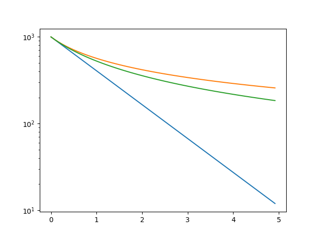
An image should be written to examples.png. We can see the hyperbolic (orange), harmonic (green), and exponential (blue) cases plotted, and the behavior looks correct (note that the vertical axis is on a logarithmic scale).
Implementation II: Fitting
Now that we can evaluate rate vs. time forecasts for given decline parameters, we need to build a way to find error-minimizing values of these parameters from observed data. This will require two things: first, a representation for the actual data to be fit; and second, a method for finding the best-fit parameters.
The first piece will come from another dataclass we’ll write to store daily oil rate data for a given well. We’ll provide this class with methods which implement best-fitting. The fitting will be accomplished using the scipy.optimize.minimize function, which provides an interface to several different optimization algorithms. Since our problem has physical bounds (for example, values of b above 2.0 don’t make sense), we’ll use the L-BFGS-B algorithm for efficient bounded optimization by a quasi-Newton method. This is a good choice for common bounded optimization problems where the bounds are independent for each variable (“box constraints”).
The specific quantity we’ll minimize is the sum of squared error (SSE) of the fit vs. the observed data. This is not necessarily the best choice of cost function, although it is certainly the most common. SSE will give high influence to the most extreme values in our data—for typical profiles, this means we’ll be much more strongly influenced by early production than late.
Absolute error (L1) functions yield more “balanced” behavior, but have awkward problems in gradient evaluation when error is near zero. There are alternative cost functions which provide the “best of both worlds”, but that’s a deep topic of it’s own—and besides, that would dip a little too deeply into “free consulting”!
During the implementation, I discovered that L-BFGS-B as implemented by scipy would occasionally try values just barely outside the bounds, which would in turn throw exceptions in the __post_init__ function of ArpsDecline. Therefore, I added an “alternate constructor” for ArpsDeclines in the form of a clamped static method, which limits parameter values precisely to the valid range.
The entire program so far, now including a class for per-well rate/time data with methods for fitting:
import numpy as np
import matplotlib.pyplot as plt # type: ignore
from scipy.optimize import minimize # type: ignore

import dataclasses as dc

from typing import List, Optional, Tuple

YEAR_DAYS: float = 365.25 # days

_GUESS_DI_NOM: float = 1.0 # nominal annual decline
_GUESS_B = 1.5

_FIT_BOUNDS: List[Tuple[Optional[float], Optional[float]]] = [
    (0.0, None), # initial rate
    (0.0, None), # nominal annual decline
    (0.0, 2.0),  # b
]

@dc.dataclass(frozen=True)
class ArpsDecline:
    qi: float # daily rate
    Di_nom: float # nominal annual decline
    b: float # unitless exponent

    def __post_init__(self):
        if self.qi < 0.0:
            raise ValueError('Negative qi')
        if self.Di_nom < 0.0:
            raise ValueError('Negative Di_nom')
        if self.b < 0.0 or self.b > 2.0:
            raise ValueError(f'Invalid b: {self.b}')

    # time (years)
    # returns (daily rate)
    def rate(self, time: np.ndarray) -> np.ndarray:
        if self.b == 0:
            return self.qi * np.exp(-self.Di_nom * time)
        elif self.b == 1.0:
            return self.qi / (1.0 + self.Di_nom * time)
        else:
            return (
              self.qi / (1.0 + self.b * self.Di_nom * time) ** (1.0 / self.b)
            )

    @staticmethod
    def clamped(qi: float, Di_nom: float, b: float) -> 'ArpsDecline':
        return ArpsDecline(
            max(qi, 0.0),
            max(Di_nom, 0.0),
            max(min(b, 2.0), 0.0),
        )

@dc.dataclass(frozen=True)
class DailyOil:
    api: str
    days_on: np.ndarray # time (days)
    oil: np.ndarray # daily rate

    def __post_init__(self):
        if len(self.days_on) != len(self.oil):
            raise ValueError('Different lengths for days on and oil rate')

    def best_fit(self) -> ArpsDecline:
        initial_guess = np.array([
            np.max(self.oil), # guess qi = peak rate
            _GUESS_DI_NOM,
            _GUESS_B,
        ])

        fit = minimize(
                lambda params: self._sse(ArpsDecline.clamped(*params)),
                initial_guess, method='L-BFGS-B', bounds=_FIT_BOUNDS)
        return ArpsDecline.clamped(*fit.x)

    # sum of squared error for a given fit to this data
    def _sse(self, fit: ArpsDecline) -> float:
        time_years = self.days_on / YEAR_DAYS
        forecast = fit.rate(time_years)
        return np.sum((forecast - self.oil) ** 2)
L-BFGS-B requires an initial guess for the value of each parameter; they don’t have to be very good guesses. We hard-code guesses for initial decline and hyperbolic exponent, and guess initial rate from the highest observed rate.
mypy doesn’t know enough about ndarrays to actually know that initial_guess and subsequent parameter arrays will unpack into exactly three floats in ArpsDecline.clamped(*params), but it’s “conservative” in the sense that if something could work, it often assumes it will, so we don’t get any warnings here.
The Optional type will come up again—it’s the exception I mentioned earlier. In mypy terms, Optional[int] is equivalent to Union[int, None]; it represents either a value of the given type or None. For example, we can write (with mypy’s blessing):
x: Optional[int]
x = 3
x = None
x = 5
We’re just about ready for our code to encounter real-world data.
Implementation III: Parsing and Converting Monthly Data
Last week we retrieved monthly volume data for Eddy County, New Mexico. I’ve extracted a subset of this data for example use, which can be found in data/eddy.zip in the project GitHub repository.
Inside the ZIP archive is a tab-separated value (TSV) file, which can be extracted to data/eddy.tsv. Each row follows the same format:
| api | year | month | oil | gas | water |
|---|---|---|---|---|---|
| 3001529417 | 1997 | 2 | 2790 | 10156 | 2353 |
| 3001529417 | 1997 | 5 | 1457 | 10155 | 2353 |
| 3001529417 | 1997 | 6 | 103 | 2449 | 322 |
| … |
The oil, gas, and water entries may each be present or absent (blank). We will only work with the oil data for our example. This file is generated by a process which sorts the data before output (in order of API, then year, then month), so we can safely assume that we are reading production well-by-well in calendar sequence.
Notice that these are monthly volumes, not daily production rates. While it’s possible to directly fit a volume vs. time (or rather, cumulative production vs. time) relation, it’s more computationally intensive. From experience, we can achieve very similar fits (within a percent or two relative error) by fitting a rate vs. time relation to monthly data, treating each monthly volume as the equivalent average daily rate, and placing its occurrence exactly half-way through the month. In addition to parsing the tab-separated file, we’ll also need to write code to handle this translation.
Real data also exposes the sorts of “anomalies” which can throw a kink in our fitting approach. Wells in real life don’t start production at a peak rate and then smoothly decline. Instead, there is generally a build-up period of increasing rate, followed by the onset of decline. The Arps equations don’t account for the “non-ideal” circumstances which cause this build-up, so we’ll need to fit only to peak-forward data. Additionally, we may choose to ignore months with production lower than a certain cutoff: these might represent operational issues which don’t reflect true reservoir performance—or, they might represent inadequate flowing pressure or other conditions which should materially affect our forecast!. This is one of many judgment calls reservoir engineers have to make when forecasting well production. For our example, we’ll implement a peak-forward data filter and a simple cutoff-based “downtime” filter.
We’ll also have to watch out for wells with too little data (after filtering) to produce a reliable fit—we’ll make this threshold configurable, but three months should be considered an absolute minimum. There’s one oddity in the OCD data which I only encountered after finishing the first draft of the program: wells with production prior to 1993 get their total volume prior to 1993 reported as a single month’s production in December 1992. This totally blows away the fitting algorithm, and in any case we don’t have a good way to recover month-by-month volumes from this lump sum, so we’ll record this value as the prior cumulative for each well (if present) and skip wells where it is present. We will also encounter some wells which, for one reason or another (recompletions, etc.) experience peak production very late in their producing histories. This will also severely violate the assumptions we make in fitting these kinds of declines, so we will detect (with a configurable cutoff) and skip these wells too.
The implementation strategy we’ll take is to create yet another dataclass for representing monthly volume records from our TSV data. This class will be the simplest yet: it’s just a “bag of data” shaped like each row of our file.
We’ll then write functions for streaming these records from a TSV file (we can use the built-in csv library to do this—please don’t reach for pandas for these kinds of simple problems!), and translating the stream of monthly records into well-by-well DailyOil objects using the averaging approach discussed previously.
The existing code for DailyOil and fitting should work fine with one or two small modifications (e.g. tracking the prior cumulative). We’ll finally write a proper main function which takes the path of a TSV file as a command-line argument, streams the data in row-by-row, fits each well if conditions are met, and plots the result to a PNG image.
The final program looks like this:
import sys
import csv
import calendar
from datetime import date, timedelta

import numpy as np
import matplotlib.pyplot as plt # type: ignore
from scipy.optimize import minimize # type: ignore

import dataclasses as dc

from typing import Iterable, Iterator, List, Optional, TextIO, Tuple

YEAR_DAYS: float = 365.25 # days
DOWNTIME_CUTOFF = 1.0 # daily rate

MIN_PTS_FIT: int = 3 # minimum # of points for fitting
PEAK_SHIFT_MAX: int = 6 # maximum # of months to peak for fitting

_GUESS_DI_NOM: float = 1.0 # nominal annual decline
_GUESS_B = 1.5

_FIT_BOUNDS: List[Tuple[Optional[float], Optional[float]]] = [
    (0.0, None), # initial rate
    (0.0, None), # nominal annual decline
    (0.0, 2.0),  # b
]

@dc.dataclass(frozen=True)
class ArpsDecline:
    qi: float # daily rate
    Di_nom: float # nominal annual decline
    b: float # unitless exponent

    def __post_init__(self):
        if self.qi < 0.0:
            raise ValueError('Negative qi')
        if self.Di_nom < 0.0:
            raise ValueError('Negative Di_nom')
        if self.b < 0.0 or self.b > 2.0:
            raise ValueError(f'Invalid b: {self.b}')

    # time (years)
    # returns (daily rate)
    def rate(self, time: np.ndarray) -> np.ndarray:
        if self.b == 0:
            return self.qi * np.exp(-self.Di_nom * time)
        elif self.b == 1.0:
            return self.qi / (1.0 + self.Di_nom * time)
        else:
            return (
              self.qi / (1.0 + self.b * self.Di_nom * time) ** (1.0 / self.b)
            )

    @staticmethod
    def clamped(qi: float, Di_nom: float, b: float) -> 'ArpsDecline':
        return ArpsDecline(
            max(qi, 0.0),
            max(Di_nom, 0.0),
            max(min(b, 2.0), 0.0),
        )

@dc.dataclass(frozen=True)
class DailyOil:
    api: str
    days_on: np.ndarray # time (days)
    oil: np.ndarray # daily rate
    prior_cum: Optional[float] # prior cumulative as of 1993/01 if available

    def __post_init__(self):
        if len(self.days_on) != len(self.oil):
            raise ValueError('Different lengths for days on and oil rate')

    def best_fit(self) -> ArpsDecline:
        initial_guess = np.array([
            np.max(self.oil), # guess qi = peak rate
            _GUESS_DI_NOM,
            _GUESS_B,
        ])

        fit = minimize(
                lambda params: self._sse(ArpsDecline.clamped(*params)),
                initial_guess, method='L-BFGS-B', bounds=_FIT_BOUNDS)
        return ArpsDecline.clamped(*fit.x)

    # filter this data set to only peak-forward production
    def peak_forward(self) -> Tuple[int, 'DailyOil']:
        if len(self.oil) == 0:
            return 0, self
        peak_idx = np.argmax(self.oil)
        return peak_idx, DailyOil(self.api,
                self.days_on[peak_idx:], self.oil[peak_idx:], self.prior_cum)

    # filter this data set to drop "downtime" (zero-production days)
    def no_downtime(self, cutoff: float = DOWNTIME_CUTOFF) -> 'DailyOil':
        keep_idx = self.oil > cutoff
        return DailyOil(self.api, self.days_on[keep_idx], self.oil[keep_idx],
                self.prior_cum)

    # sum of squared error for a given fit to this data
    def _sse(self, fit: ArpsDecline) -> float:
        time_years = self.days_on / YEAR_DAYS
        forecast = fit.rate(time_years)
        return np.sum((forecast - self.oil) ** 2)

@dc.dataclass(frozen=True)
class MonthlyRecord:
    api: str
    year: int
    month: int
    oil: Optional[float]
    gas: Optional[float]
    water: Optional[float]

def month_days(year: int, month: int) -> int:
    return calendar.monthrange(year, month)[1]

def mid_month(year: int, month: int) -> date:
    return date(year, month, 1) + timedelta(days=month_days(year, month) / 2)

# precondition: monthly is sorted by API then date
def from_monthly(monthly: Iterable[MonthlyRecord]) -> Iterator[DailyOil]:
    last_api: Optional[str] = None
    first_prod: Optional[date] = None
    prior_cum: Optional[float] = None
    days_on: List[float] = list()
    oil: List[float] = list()

    for m in monthly:
        if m.api != last_api:
            if last_api is not None:
                yield DailyOil(last_api, np.array(days_on), np.array(oil),
                        prior_cum)
                days_on = list()
                oil = list()
            last_api = m.api
            first_prod = None

        # NM OCD reports cumulative prior to 1993-01-01 as 1992/12 monthly
        if m.year == 1992 and m.month == 12:
            prior_cum = m.oil
            continue

        if first_prod is None:
            first_prod = date(m.year, m.month, 1)

        if m.oil is not None: # skip months with missing oil data
            days_on.append((mid_month(m.year, m.month) - first_prod).days)
            oil.append(m.oil / month_days(m.year, m.month))

    if last_api is not None:
        yield DailyOil(last_api, np.array(days_on), np.array(oil), prior_cum)

def float_or_none(val: str) -> Optional[float]:
    if val == '':
        return None
    return float(val)

def read_production_file(prod_file: TextIO, header: bool = True, **csvkw
        ) -> Iterator[MonthlyRecord]:
    reader = csv.reader(prod_file, **csvkw)
    if header:
        next(reader) # skip header row

    for (api, yr, mo, o, g, w) in reader:
        yield MonthlyRecord(api, int(yr), int(mo),
                float_or_none(o), float_or_none(g), float_or_none(w))

def main(argv: List[str]) -> int:
    if len(argv) != 2:
        print(f'Usage: {argv[0]} production-file', file=sys.stderr)
        return 1

    with open(argv[1], 'r', newline='') as production_file:
        data = read_production_file(production_file, delimiter='\t')
        for well in from_monthly(data):
            if well.prior_cum is not None:
                print(f'{well.api}: production prior to 1993',
                        file=sys.stderr)
                continue

            shift, filtered = well.peak_forward()
            if shift > PEAK_SHIFT_MAX:
                print(f'{well.api}: peak occurs too late for fitting',
                        file=sys.stderr)
                continue

            filtered = filtered.no_downtime()
            if len(filtered.days_on) < MIN_PTS_FIT:
                print(f'{well.api}: not enough data', file=sys.stderr)
                continue

            plt.semilogy(filtered.days_on, filtered.oil)
            best_fit = filtered.best_fit()
            plt.semilogy(well.days_on, best_fit.rate(well.days_on / YEAR_DAYS))
            plt.savefig(f'plots/{well.api}.png')
            plt.close()

    return 0

if __name__ == '__main__':
    sys.exit(main(sys.argv))
Our peak-forward and downtime filters return new DailyOil objects: remember, we’ve made our classes immutable (frozen), so (just like in functional programming languages) we return altered copies of objects rather than mutate their internal state. This also has the advantage of ensuring that the original, unaltered, data sticks around for comparison!
The “mid-month” logic uses Python’s built-in libraries for date and time manipulation. Everything is done on a “calendar month” basis, which is just to say that by contrast to certain software tools, we actually recognize the fact that “30 days hath September” when translating monthly volumes to daily average rates.
The read_production_file and from_monthly functions are interesting in that they take advantage of Python’s support for generators to achieve streaming processing of the input data. Remember, the input file may be very large, but to fit one well at a time we need at most enough memory to store that specific well’s production data. Rather than read the TSV file “eagerly” to a list, we yield rows one at a time. The from_monthly function takes advantage of the known ordering of the rows to yield one well’s worth of production at a time.
main’s type signature is like C’s int main(int argc, char *argv[]): we take a list of command-line arguments and return an exit status to the operating system.
Results
We can run the program against our example file (remember to typecheck first!):
mypy pydca.py
python pydca.py data/eddy.tsv
This will generate warning messages about any skipped wells, and write per-well plots to the plots/ directory.
On my workstation, this runs in a minute or two against the all-Eddy-County data set (this is excerpted in the GitHub repository) and produces fits for 251 wells (with many others skipped due to the criteria we imposed). This performance is, in my opinion, adequate for a reservoir engineering or evaluation “quick look” workflow. We could do better, but that’s a deep topic for another time.
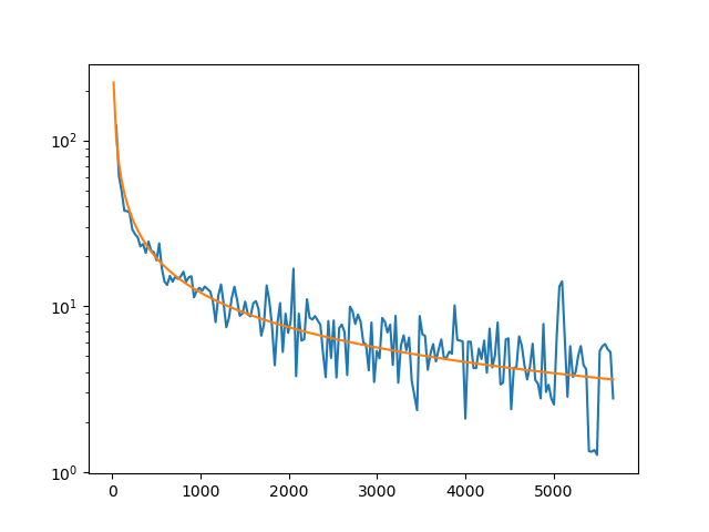
How do the fits look? They’re OK. Some look quite good:
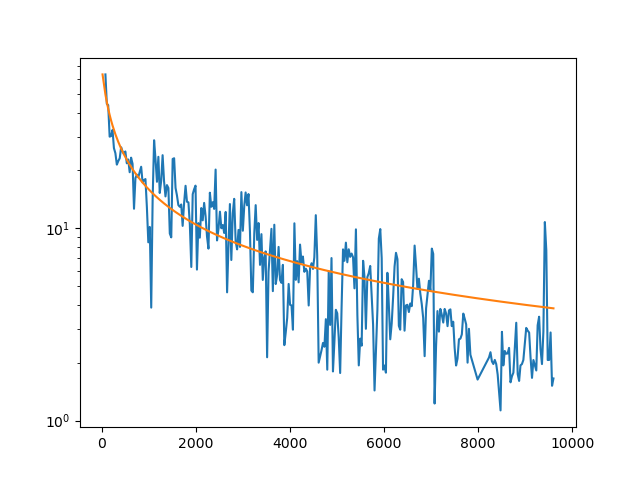
Others look pretty poor, and might reflect flaws in the data or in our filtering process. On the other hand, 20 barrels per day isn’t much of a well to worry about anyway!
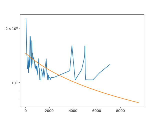
Finally, some hint at the limitations of basic Arps decline curves which I mentioned previously. Even though the absolute volumes are low, I’d argue that this fit overstates reserves because the late-time behavior has a distinctly “steeper” character than the early-time behavior. We should probably consider one of the many models which allow for fitting multiple flow regimes, which is a great topic to consult a reservoir engineer about, or your favorite consultant.